
Damien Decremer joined ECMWF in 2014 after completing a PhD in climate science and statistics in Korea.
Modelling, computing and statistics come together in Earth system model diagnostics and calibration work. ECMWF scientist Damien Decremer has the required interdisciplinary expertise.
His first passion was computing: at the age of 15, he used the Python programming language to recode the interface of a video game he liked.
However, after completing a Masters in electronic engineering, he did not see his professional future in optimising electronic devices and reconsidered his career options.
“While travelling during a gap year I met a professor in Korea who invited me to do a PhD in climate science and statistics, and I agreed,” he recalls.
This set him on course for a position in ECMWF’s Earth System Predictability Section, where he worked on land surface model initialisation and seasonal forecast verification and diagnostics.
Since then he has moved to the Environmental Forecasts team and has added flood model calibration to his growing portfolio. In each of these activities, his computing and statistical skills have proved extremely useful.

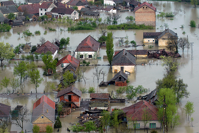
Seasonal and flood forecasts are of interest to a wide range of users, including emergency services and businesses in a range of sectors. (Photo: SlobodanMiljevic/iStock/Thinkstock)
Helping with the seasonal verification suite
A forecasting system is not very useful if nobody knows how good it is. That is why continuous forecast verification is part and parcel of operational numerical weather prediction.
Verification is also a first step towards diagnostics: an assessment of where errors in forecasts come from and how they can be remedied.
“When I joined ECMWF, the seasonal forecast verification software suite needed modernising: it had evolved a lot over time and had become difficult to run and maintain,” Damien says.
“The suite was made up of lots of disconnected scripts. I was able to apply my computing skills to integrate these bits and pieces into a ‘seasonal verification suite’, which can be used to verify seasonal experiments. This suite has been very helpful for the development of the new seasonal forecasting system SEAS5.”
Damien also used his statistical skills to add the widely used CRPS skill score to this suite.

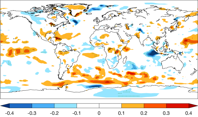
In November 2017, ECMWF implemented the latest generation of its seasonal forecasting system, SEAS5. It improved forecasts in the tropics, in particular for sea-surface temperature in the equatorial Pacific. The chart shows the difference in CRPSS between SEAS5 and its predecessor, S4, for ensemble mean 2-metre temperature predictions for June–July–August from 1 May. A CRPSS difference of 1 corresponds to a 100% improvement in skill. (Figure reproduced from doi:10.5194/gmd-2018-228 under CC-BY-4.0)
Seasonal forecast spread conundrum
An example illustrates why an in-depth understanding of statistics can be vital to be able to interpret verification results correctly.
ECMWF’s seasonal forecasts are ensemble forecasts. This means that a number of forecasts are run simultaneously with slightly different initial conditions and slightly different model realisations.
The spread in the ensemble members gives an indication of uncertainty in the forecast. A large spread means large uncertainty or low confidence, and a small spread small uncertainty or high confidence.
Or at least that’s the way it should be if the ensemble forecast system has been set up correctly.
One of the verification scores used, known as the Ratio of Predictable Components (RPC), suggests that in many forecasting systems the spread in wintertime seasonal forecasts for the North Atlantic region is unnecessarily large: the forecasts seem to be underconfident.
However, another verification measure, the error–spread relationship, suggests that the spread is just right. Damien helped to investigate this issue within ECMWF’s seasonal forecasting system.
“We had to delve deep into the behaviour of the mathematics of the scores, and to look at time series spanning many decades, to realise that the RPC score is very sensitive to the temporal sampling.” Damien says.

Over a sufficiently long period, RPC and the ratio of root-mean-square error (RMSE) and ensemble spread are on average close to 1, which means that the seasonal forecasting system is neither underconfident nor overconfident.
River network resolution
One of Damien’s first tasks in the Environmental Forecasts team was to investigate how to improve the resolution of the river network in the flood model used by the European Flood Awareness System (EFAS).
At 5 km grid spacing, it is too coarse to accurately represent hills and valleys, so that in the model rainwater might flow into the wrong river basin.
The low resolution also means that more than one river might flow into and out of one and the same grid box.
“In the model, each grid box has only one outflow, so the system cannot cope with two rivers entering and exiting one and the same grid box through different edges. The model would think that they merge into a single river,” Damien explains.
But resolution cannot be increased at will: it is constrained by computational and data flow capacity and the need to produce forecasts in a timely manner.
“We found that representing the river network at 1 km grid spacing is a great improvement on 5 km and computationally feasible. However, manually increasing the river network resolution over a large domain is impossibly time-consuming. That is why we are developing a complex algorithm to automate the process.”

Representing the river network at 1 km grid spacing enables more realistic hydrological modelling than a grid spacing of 5 km. The coloured squares show how the model sees the rivers.
Flood model calibration
An even bigger project Damien is working on is the implementation of a new calibration tool in EFAS.
Flood modelling involves the use of a range of parameters which are not precisely known, relating to how rainwater drains into river basins and lakes.
Experiments can be carried out to see how these parameters need to be adjusted to optimise flood simulations.

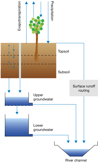
A hydrological model takes into account parameters such as the snowmelt coefficient, soil infiltration rate and surface runoff coefficient to help model the processes that determine the magnitude of the flow in a river channel.
“It’s an iterative process based on machine learning,” Damien explains. “One approach is to run historical simulations with a certain range of parameters, a bit like an ensemble, and then to select the parameters that produce the best fit with observations. Then we modify those parameters slightly to generate a new ensemble of simulations, and so on, until optimal values are found. We then apply those parameter values in future forecasts.”
Damien has found that his skills in computing and statistics complement those of the modellers in his team very well. As he and his team investigate ways to improve the calibration, his statistics background will be very helpful.
“One should never be afraid of plunging into the unknown using an interdisciplinary approach. It often leads to interesting new insights and in my case it has transformed my professional life.”
