
Successful weather forecasts start from accurate estimates of the current state of the Earth system. Such estimates are obtained by combining model information with Earth system observations in a process called data assimilation. Recent work at ECMWF has demonstrated for the first time that assimilating cloud observations from satellite radar and lidar instruments into a global, operational forecasting system using a 4D-Var data assimilation system is feasible and improves weather forecasts.
Motivation
Cloud‐related satellite radiance observations have been at the forefront of recent advances in data assimilation at ECMWF. However, one weakness of these new observations is that they contain limited information on cloud structure, which can lead to ambiguities in the positioning of clouds in the model. Active observations from profiling instruments, such as cloud radar or lidar, contain a wealth of information on the vertical structure of clouds and precipitation but have never been assimilated in global numerical weather prediction (NWP) models. Currently there are no fully functioning space‐borne radar or lidar instruments, but historical observations from CloudSat and CALIPSO (Cloud‐Aerosol Lidar and Infrared Pathfinder Satellite Observations), part of the NASA A‐train constellation, are useful datasets for feasibility studies. In the next few years, new satellite missions with cloud radar and lidar are planned, such as EarthCARE (Earth, Clouds, Aerosols and Radiation Explorer) from the European Space Agency (ESA) and the Japan Aerospace Exploration Agency (JAXA), which has been described by Illingworth et al. (2015).
Previous studies, in particular the STSE Study funded by ESA (Janisková, 2014), have indicated that observations of clouds from space‐borne radar and lidar are not only useful to evaluate NWP model performance, but that they also have potential for use in assimilation to improve the initial atmospheric state (the analysis). The studies have demonstrated that a two‐step technique which combines one‐dimensional (1D‐Var) with four‐dimensional (4D‐Var) data assimilation, where radar reflectivity and attenuated backscatter profiles are indirectly assimilated via pseudo‐observations of temperature and humidity, can improve the analysis and forecasts (Janisková, 2015).
Inspired by the success of these previous studies, the ECMWF 4D‐Var system has been adapted to enable the direct assimilation of radar and lidar observations. The direct (in‐line) data assimilation and monitoring systems were developed during the most recent ESA project on EarthCARE assimilation (Janisková & Fielding, 2018). 4D‐Var assimilation experiments have been performed using CloudSat cloud radar reflectivity and CALIPSO lidar backscatter. Using the full system of regularly assimilated observations at ECMWF, several experiments have been carried out in which these observations were added to the system. This is the first time that the feasibility of assimilating such observations directly into a global‐scale 4D‐Var system has been demonstrated. The results are promising, with improvements in forecast skill shown for temperature, wind and the model radiation budget. Selected results from this encouraging study are presented here.
Prerequisites
To prepare the data assimilation system for the new observations of cloud radar reflectivity and lidar backscatter, several important developments were required. First, there had to be a reasonable representation of the physical processes related to the observations, such as moist processes related to large‐scale and convective cloud formation, as well as an ‘observation operator’ providing realistic model equivalents to the observations (see Box A).
Second, to handle observations appropriately in the data assimilation system, quality control and screening as well as a bias correction scheme are required. The quality control for the cloud radar and lidar observations is based on thresholds for indicators of signal strength; first‐guess departures (the differences between observations and the short‐range forecasts used in the data assimilation system, called the ‘first guess’); estimated total attenuation; and, for radar, expected multiple scattering. The bias correction is based on a climatology of first‐guess departures, covering a period when the observations were passively monitored. To provide an implicit regime dependence, the bias correction depends on temperature and height. Another important component of the system is the definition of the errors assigned to observations. The assumed observation errors take into account instrument errors, observation operator errors, and representativeness errors due to the narrow field of view, as described in Box B.
A
The observation operator
A prerequisite for the assimilation of any type of observation is that the model must be able to simulate the observations with a sufficient degree of realism. For remote‐sensing observations of clouds, this means that the model must be able to represent the physical properties of clouds (e.g. their water content) and their appearance as seen from a particular remote‐sensing instrument. In the case of height‐resolved measurements, the model must also be sufficiently accurate in assigning the correct (or close enough) altitude to clouds.
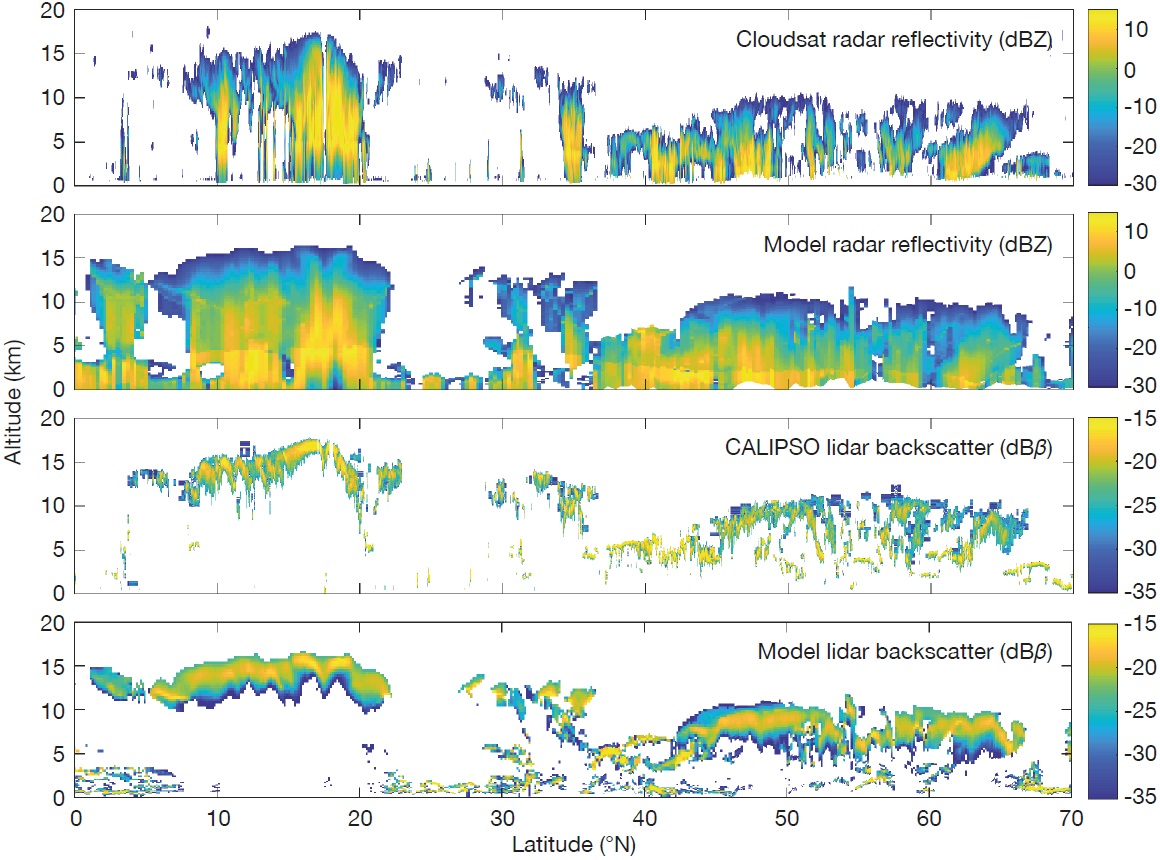
The observation operators used for CloudSat and CALIPSO are similar and follow the same overall method. For each radar or lidar profile, the nearest model profile is used as input to a look‐up table that contains pre‐computed scattering and extinction properties according to hydrometeor mass, type and temperature. These scattering properties are then used as input to a radiative transfer calculation to obtain the model equivalent radar reflectivity or lidar attenuated backscatter. Optional features include the simulation of multiple scattering (where after their first scattering event, photons either remain within the instrument field‐of‐view or return to it at a subsequent scattering event) and the representation of the sub‐grid variability of clouds.
As an example, the figure shown below shows the performance of the observation operators for an A‐train track on 15 September 2009 over the Pacific Ocean and Japan that includes a direct overpass of Typhoon Choi‐wan including its eyewall. The overall performance of the model is very good: many of the cloud features shown by the observations are present in the model equivalents. The figure also shows how the lidar provides mostly information on ice cloud and liquid cloud top height as the signal attenuates very quickly. The radar provides more information on vertical structure and is only completely attenuated in deep convection, such as in the rain bands close to the typhoon eyewall.
Experimental setup
In our study, measurements of cloud radar reflectivity from the CloudSat 94 GHz radar and of lidar backscatter due to clouds at 532 nm from CALIPSO have been assimilated in the 4D‐Var system. Using the full system of regularly assimilated observations at ECMWF, several assimilation experiments have been performed using ECMWF’s 4D‐Var data assimilation system for the three‐month period from 1 August 2007 to 31 October 2007, at a horizontal resolution of TCo639 (corresponding to a grid spacing of approximately 18 km on a cubic octahedral grid) and 137 vertical levels.
Many different experiments have been performed to understand the new observation type, such as using different combinations of observations (radar only; lidar only; or both observations in combination with all other assimilated observations), different observation errors (different degrees of error inflation) or observation reduction (increased horizontal averaging or vertical thinning). Here, we present the results from only one of the experiments. In that experiment (EXP), on top of all other normally assimilated observations, both cloud radar reflectivity and lidar backscatter were assimilated using double observation errors compared to the ones estimated in Janisková & Fielding (2018), also described in Box B, and applying observation reduction by horizontal averaging of cloud radar and lidar observations to the coarser resolution of 72 km. For comparison, a control experiment (CTR) was carried out with all regularly assimilated observations, but without the new cloud radar and lidar observations included in the 4D‐Var system. Ten‐day forecasts were run from the analyses to study the impact of the new observations not only on the analysis but also on forecasts.
Results
The first step in evaluating the impact of assimilating cloud radar reflectivity and lidar backscatter is to compare the resulting analysis against these observations. This evaluation showed that the analysis is closer to cloud radar and lidar observations than would be the case if these observations were not assimilated. The fact that the analysis is drawn to the radar and lidar observations can be seen in Figure 1, where the impact of observations of individual clouds can be assessed. For example, in the analysis, both the structure of the precipitation within the warm front of the North Sea cyclone and the ice cloud in the Atlantic Cyclone south of Greenland are brought closer to the observations.

B
Observation errors
In addition to the observations, a key input into a data assimilation system is the estimated error of the observations. The observation error, in combination with the error in the short‐range forecasts used in the data assimilation system, controls the weight of the observations in producing the analysis. In 4D‐Var, the observations are assumed to be unbiased and their random error is assumed to be normally distributed. At ECMWF, many observations are assigned a static error based on the instrument error and/or first‐ guess departure statistics. For profiling observations of clouds, the observation error tends to be much more situation dependent and warrants a more complex approach.
To characterise the observation error for the radar and lidar observations, we take an ‘error inventory’ approach, where individual components of the observation error are specified before being squared and added together (assuming no correlation). The three main sources of error accounted for are instrument error, observation operator error and representativeness error. The figure below provides a breakdown of the different sources of observation error for the same CloudSat A‐train track as in Box A. In this figure, the observed radar reflectivity has been averaged to a grid spacing of about 18 km. However, in the experiments presented in this article we used a coarser grid spacing of about 72 km.
For the radar observations, the greatest source of error is the representativeness error, which accounts for the mismatch of scales between the narrow footprint of the observations and the model. To quantify the error, we combine the along‐track variability in the observations with a climatological correlation function (Fielding & Stiller, 2019). The greatest representativeness error tends to be found in convective situations; note the increase in error around the typhoon’s eyewall at 17°N. The second largest source of error is the observation operator error. This is computed using a Monte Carlo approach, by perturbing the microphysical assumptions (such as particle size distribution and particle scattering properties) in the observation operator. The smallest errors tend to be in the middle of clouds and the largest in regions of strong attenuation. Finally, the smallest component of the overall error is the instrument error, which is calculated dynamically using the instrument signal‐ to‐noise ratio. Away from cloud edges, the instrument error tends to be dwarfed by the other errors.
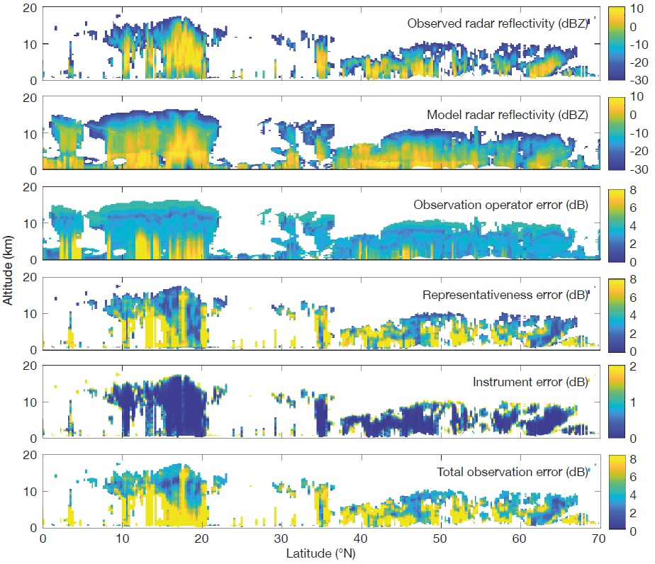
Figure 2 compares first‐guess departures with analysis departures (the differences between observations and the analysis) with respect to CloudSat cloud radar reflectivity (Figure 2a) and CALIPSO cloud lidar backscatter (Figure 2b). The plots confirm that EXP produces an analysis that is closer to cloud radar and lidar observations than the first‐guess. The results also indicate that the analysis is drawn less strongly to cloud lidar observations than to cloud radar observations, perhaps due to the stronger attenuation of the lidar signal, which can lead to ambiguities in the true cloud amount. Investigations are planned to assess whether assimilating the whole profile rather than just when there is cloud in both the model and the observations might help to solve this deficiency.


The impact of assimilating radar and lidar observations on the analysis has also been assessed by comparing the fit of the first guess to other assimilated observations for the same three‐month period (Figure 3). The comparison of the first‐guess departures between EXP and CTR indicates a slight improvement with respect to satellite temperature observations as seen for both tropospheric and stratospheric channels of the AMSU‐A instrument (Figure 3a), as well as for HIRS instrument channels 5–8 and 13–15, which are sensitive to temperature (Figure 3b). An evaluation with respect to wind observations indicates a generally small degradation at around 1,000 hPa, which is more pronounced when comparing the first guess with SATOB wind observations (atmospheric motion vectors). For the levels above, the impact of the new observations on the analysis is broadly neutral when checked against satellite observations, but slightly positive and increasingly better higher up in the troposphere when evaluated with respect to conventional wind observations (such as TEMP, PILOT, AIREP and wind profilers). Overall, verification against other assimilated observations has shown that first‐guess departures are either unchanged or slightly reduced when assimilating the new observations.
The impact of the assimilation of cloud radar and lidar observations on the skill of forecasts has been evaluated by verifying forecasts against each experiment’s own analysis, as well as against other assimilated and some independent observations (i.e. observations not used by the assimilation system).
Figure 4 shows the impact of assimilating space‐borne cloud radar and lidar observations on forecasts up to 10 days ahead over the whole globe for the three‐ month period from August to October 2007. For temperature, the largest improvement in forecast skill is observed in the lowest levels (especially at 1,000 hPa), while the impact is close to neutral at 850 hPa and above. Similarly, there is a marginally positive impact at 1,000 hPa for relative humidity. Globally, slight improvements in forecast skill for vector wind are most pronounced at the model levels 500 hPa and above. The skill of geopotential forecasts is slightly improved across all levels in EXP. Although one could argue that the overall impact, albeit positive, is rather small, it is important to note that the results presented here are the first ever results of direct 4D‐Var assimilation of cloud radar and lidar observations without any extensive tuning. Such tuning is necessary for any new types of observations to be included operationally in the data assimilation system. Therefore, these results are encouraging, but more experiments are needed to further improve the impact of these observations.


A further promising result shows that the model radiation budget can be improved by assimilating cloud radar and lidar observations. This was revealed by verification of the forecast against fully independent observations of the net top‐of‐atmosphere (TOA) short‐wave radiation from CERES (Clouds and the Earth’s Radiant Energy System) instruments for the period of August 2007. Figure 5 shows that for EXP the forecast of TOA short‐wave radiation is improved up to 60 hours ahead. When looking at day 1 forecasts, there is a positive impact up to 200 km from the A‐train track. As expected, the impact diminishes with greater distance from the satellite track.
Summary and prospects
The assimilation studies presented in this article have demonstrated the potential benefits of assimilating space‐borne radar and lidar observations for NWP. The experiments, which cover a period of three months, have shown promising results. Firstly, ECMWF’s 4D‐Var system provides analyses closer to cloud radar and lidar observations than would be the case if these observations were not assimilated. Secondly, including cloud radar reflectivity and lidar backscatter observations in the 4D‐Var system was found to have a positive impact on both the analysis fit to other observations and the subsequent forecast. Increasing forecast skill by including new observations in a well‐established observing system is extremely difficult, so these encouraging results warrant further research to maximise the direct benefit of cloud radar and lidar assimilation.
The results presented were found to be sensitive to observation error. As a result, it is envisaged that further gains in forecast skill could be achieved through careful tuning. The correlation of observation error, particularly in the vertical, should also be considered. The behaviour of the assimilation system for different regimes, for example the effect of cloud radar and lidar in convective situations, requires further work and could benefit from improvements in the observation operator assumptions or screening criteria. Another line of potentially very fruitful research is to investigate how cloud radar and lidar observations can support the assimilation of other observation types sensitive to clouds, in particular in the all‐sky radiance assimilation framework used operationally at ECMWF. By assimilating the vertical profile of clouds, ambiguity in the height and depth of clouds could be removed, which could improve the impact of the radiance observations.
Further reading
Fielding M. & O. Stiller, 2019: Characterizing the representativity error of cloud profiling observations for data assimilation. J. Geophys. Res. - Atmospheres, 124, 4086– 4103.
Illingworth, A., H.W. Barker, A. Beljaars, M. Ceccaldi, H. Chepfer, N. Clerbaux, J. Cole, J. Delanoë,
C. Domenech, D.P. Donovan, S. Fukuda, M. Hirakata, R.J. Hogan, A. Huenerbein, P. Kollias, T. Kubota, T. Nakajima, T.Y. Nakajima, T. Nishizawa, Y. Ohno, H. Okamoto, R. Oki, K. Sato, M. Satoh, M.W. Shephard, A. Velázquez-Blázquez, U. Wandinger, T. Wehr & G.J. van Zadelhoff, 2015: The EarthCARE Satellite: The Next Step Forward in Global Measurements of Clouds, Aerosols, Precipitation, and Radiation. Bull. Am. Meteorol. Soc., 96 (8), 1311–1332, doi:10.1175/BAMS‐D‐12‐00227.1.
Janisková, M., 2014: WP‐3200 report: Assimilation experiments for radar and lidar – Support‐to‐Science‐Element (STSE) Study EarthCARE Assimilation, ECMWF Contract Report to the European Space Agency .
Janisková, M., 2015: Assimilation of cloud information from space‐borne radar and lidar: Experimental study using 1D+4D‐Var technique. Q. J. R. Meteorol. Soc., 141, 2708–2725, doi:10.1002/qj.2558.
Janisková, M. & M. Fielding, 2018: Operational Assimilation of Space‐borne radar and Lidar Cloud Profile Observations for Numerical Weather Prediction, ECMWF Contract Report to the European Space Agency .