
Two years ago, forecasting systems were predicting the development of a potentially major El Niño – a warming of the equatorial Pacific Ocean which has impacts on weather patterns around the world. The 2015/16 El Niño turned out to be in the same class as the biggest such events recorded in the 20th century. Its evolution was well predicted by ECMWF forecasts as well as by EUROSIP multi-model forecasts. The latest forecasts for 2017 at the time of going to press are indicating the possibility of another El Niño developing later this year. El Niño is the warm phase of the El Niño Southern Oscillation (ENSO). The cool phase is known as La Niña.
To illustrate our El Niño forecasting capabilities, we review the major event that occurred in 2015/16: what happened in the tropical Pacific and how well was it predicted? We show that the event contributed to successful seasonal forecasts of European winter temperatures, and we discuss the latest El Niño forecasts (March 2017), both from ECMWF and from the multi-model EUROSIP system.
The evolution of the 2015/16 El Niño
The two strongest El Niños of the 20th century were those of 1982/83 and 1997/98, each of which was considered at the time a ‘once-in-a-century’ event. The El Niño of 2015/16 is in the same class as those of 1982/83 and 1997/98, and it set new records in the NINO4 and NINO3.4 regions in the western and central Pacific.
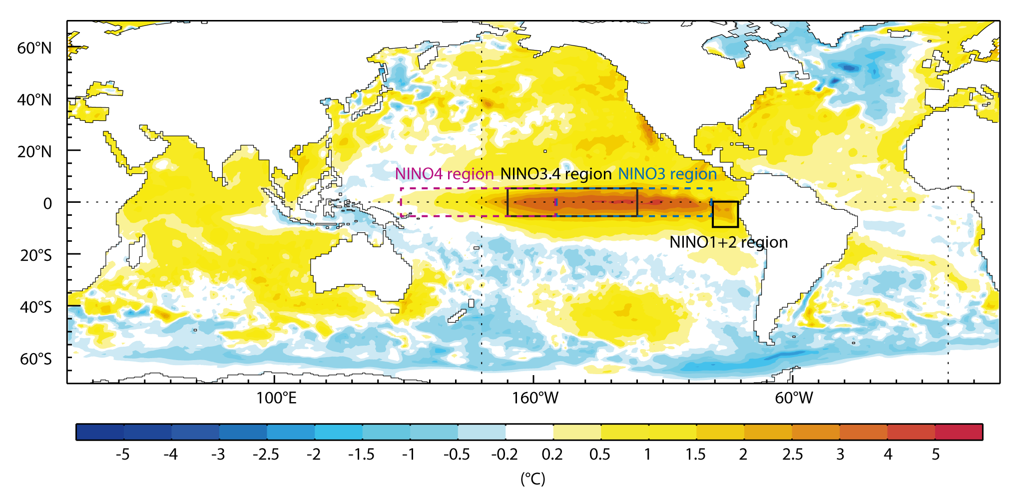
Figure 1 shows the spatial structure of the El Niño at its peak in November 2015. The vast extent of the event – more than 10,000 km in zonal (east–west) extent – and its ability to influence the deep tropical convection that drives the general circulation of the atmosphere is what gives El Niño its global impact. El Niño variability is generally monitored by the use of indices, calculated from average sea-surface temperatures (SST) over the regions marked on the map. NINO3.4, covering the central region of the equatorial Pacific, is most commonly used as a measure of the overall strength of an ENSO event.

The 2015/16 El Niño can best be understood by looking at the evolution of NINO3.4 SST (Figure 2). In a normal year, there is a pronounced seasonal cycle in SST, as indicated by the red line. El Niño conditions are normally monitored as anomalies with respect to this mean seasonal cycle. At the beginning of 2015, the equatorial Pacific was already warm, as a leftover from borderline El Niño conditions which developed during 2014. The SST warmed at the usual rate during March, but continued warming through April and into May, with temperatures approaching 29°C. Normally, the ocean surface cools from June to September, as zonal winds strengthen and upwell cooler water at the equator, but in 2015/16 equatorial waters stayed warm for a whole year, with peak temperatures reached in November. Thus the usual seasonal cycle was completely upended. Due to the nature of the coupling between ocean and atmosphere in the equatorial Pacific, this dramatic change in SST was both a symptom and a cause of corresponding major changes in atmospheric winds and precipitation patterns.
The 2015/16 El Niño broke warming records in the central Pacific, represented by the NINO3.4 and NINO4 indices. At its peak in November 2015, the NINO3.4 SST anomaly reached 3.0°C, breaking the previous record of 2.8°C set in January 1983. In the NINO4 region, large positive anomalies are hard to achieve because average conditions are already warm. In 2015, the anomaly reached 1.7°C, a substantial increase of 0.4°C on the previous record, set in 2009. SST analyses become less precise going back in time, but the size of the anomalies in NINO4 and NINO3.4 means we are fairly confident that these are record values for the whole of the observational period back to 1860. By contrast, in the eastern Pacific (monitored by indices for the NINO3 and NINO1+2 regions) the El Niño remained below the level of the 1982/83 and 1997/98 events. It must be borne in mind that the anomaly records depend on the reference climate, which in this case is a 30-year climate (1981–2010).
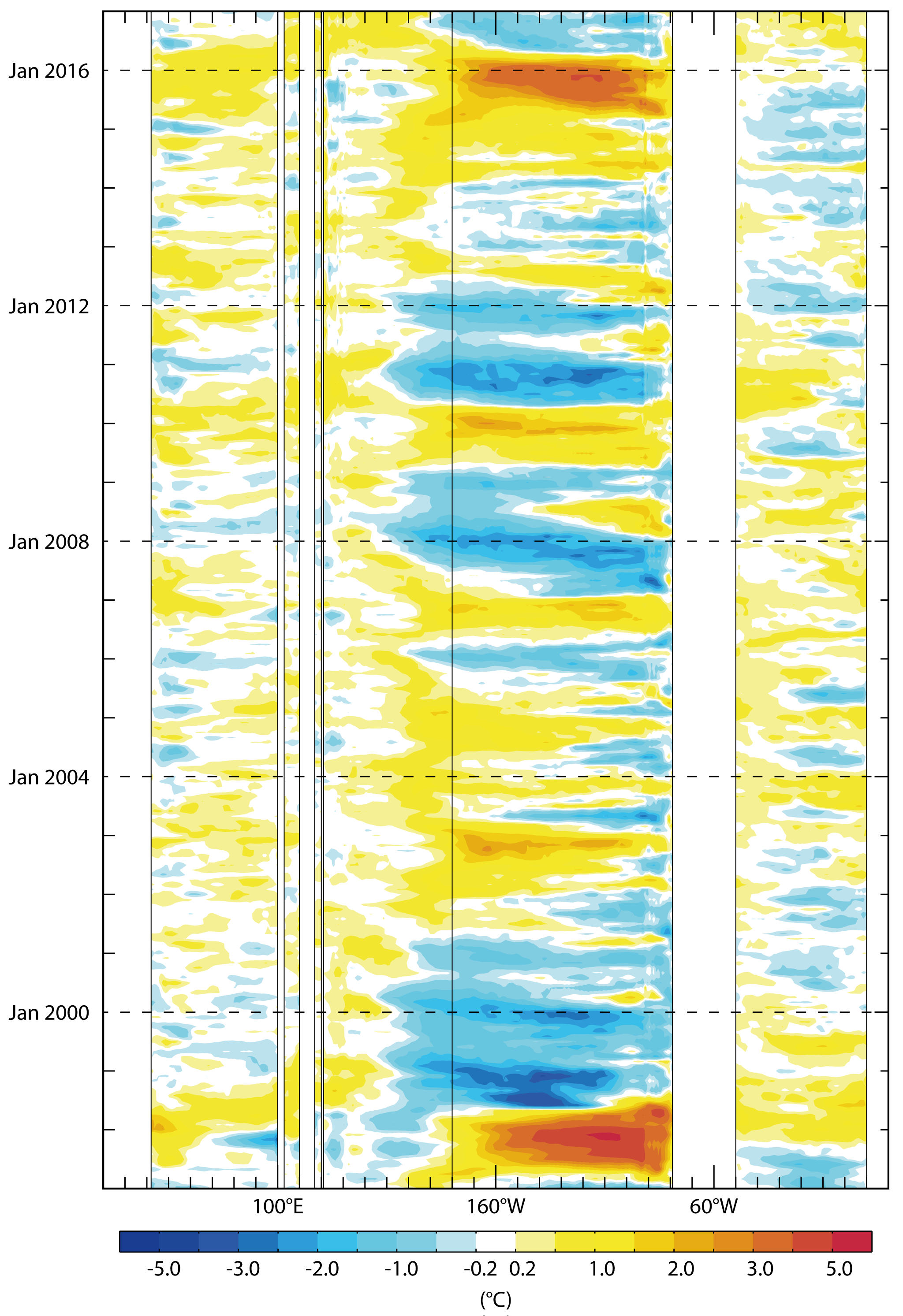
Figure 3 puts the current event in the context of the last 20 years. It shows the evolution of SST anomalies at the equator from January 1997 (bottom) to December 2016 (top), with conspicuous spikes in 1997/98 and at the end of 2015. It shows that at the equator the 2015/16 event was exceptionally strong, but not quite as strong as 1997/98. The peak warm anomalies were not so long-lived either, decaying quickly after November 2015. The aftermaths of the events are also remarkably different: 1997/98 was followed by an intense and long-lived cold La Niña episode, while the 2016 La Niña has been weak and short-lived. In between, the chart shows fluctuations between warm El Niño conditions and colder La Niña episodes in the central and eastern Pacific.
How well was the 2015/16 El Niño predicted?

Forecasts in March 2015 suggested the possibility of a substantial El Niño event developing later that year (Stockdale, 2015). Figure 4 shows a series of ECMWF ensemble forecasts from 1 March, 1 August and 1 November 2015 for SST anomalies with respect to the 1981 to 2010 climate in the NINO3.4 region. They demonstrate a close match between the predicted and observed SST tendencies. The forecast from 1 March correctly predicted the observed warming between March and September, although there was a large spread of possible outcomes, indicating great uncertainty, at longer lead times. It is well known that between March and May the predictability of El Niño is low. The forecast from 1 August captured the timing of the peak of the warming that occurred at the end of the year, and its incipient decline. However, most ensemble members overestimated the peak magnitude. Finally, the 1 December forecast correctly and confidently predicted a rapid fall in SST anomalies during the next six months, although the predicted decline between December 2015 and February 2016 is too steep. The ensemble prediction suggested that uncertainty was relatively low as the spread is relatively small even at longer lead times.
Experience has shown that, at seasonal timescales, the most reliable forecasts are obtained by combining and calibrating the output from a number of independent forecasting systems. At ECMWF, output from four major forecasting centres (ECMWF, the UK Met Office, Météo-France and NCEP, the US National Centers for Environmental Prediction) is combined to make the EUROSIP multi-model products. EUROSIP calibrated NINO plumes show a probability distribution computed from the ensemble with a weighting that takes into account the reliability of each model. The distribution is plotted showing the 2nd, 10th, 25th, 50th, 75th and 98th percentiles of the distribution.

Figure 5 shows the EUROSIP probability spread of SST anomalies in NINO3.4 forecasts from 1 March 2015, 1 August 2015 and 1 December 2015. It shows that, here too, the broad evolution of the anomalies was well predicted, especially in the 1 August forecast. For much of the forecast period in the 1 March forecast, the observed SST anomaly lies beyond the 75th percentile. In the EUROSIP forecast from 1 December, the predicted decline in anomalies was again too steep in the first two months, and the observed anomalies were beyond the 98th percentile in February and March.
Overall, both the ECMWF and EUROSIP forecasts successfully predicted the timing of the onset, peak and decline of the 2015/16 El Niño event. The intensity was also captured fairly well albeit with a large uncertainty at longer lead times, especially in the 1 March and 1 August forecasts.
El Niño and European seasonal forecasts
Seasonal forecasts provide global information about atmospheric and oceanic conditions averaged over the next few months. Despite the chaotic nature of the atmosphere, such long-term predictions are possible because some climate phenomena show variations on timescales of seasons or years and are, to a certain extent, predictable. The most important of these phenomena is the ENSO cycle.
Useful web links
ECMWF and EUROSIP ENSO forecasts are available on ECMWF’s website: http://www.ecmwf.int/en/forecasts/charts
Information on the EUROSIP multi-model forecasting system can be found here: http://www.ecmwf.int/en/forecasts/documentation-and-support/long-range/seasonal-forecast-documentation/eurosip-user-guide/multi-model
For more information on the Copernicus Climate Change Service’s prototype seasonal forecast products, visit: http://climate.copernicus.eu/seasonal-forecasts
Although ENSO is a coupled ocean–atmosphere phenomenon centred over the tropical Pacific, its fluctuations affect the climate in other parts of the globe. During an ENSO event, the enhanced convection over the warm waters in the central and eastern tropical Pacific triggers changes in the strength of the Hadley circulation, leading to modifications in circulation patterns worldwide including, for example, the position of the jet stream that flows from west to east over the North Pacific in winter months. By strengthening the Hadley circulation, ENSO can trigger a cascade of deviations from normal rainfall and temperature patterns around the globe. These remote impacts are called ENSO teleconnections. ENSO teleconnection patterns are reflected in historical observations and are the basis of any empirical model.
The predictive skill of any dynamical model is strongly associated with the ability to accurately reproduce ENSO teleconnections. It follows that in years when ENSO is active, seasonal predictions are expected to be more accurate than in years when ENSO is in neutral conditions.
The year 2015 was hotter than any previous year in global datasets going back more than 130 years. Global near-surface temperature was well over 0.4°C warmer than the 1981–2010 average and almost 0.1°C warmer than the previous warmest year. The year 2016 was in turn nearly 0.2°C warmer than 2015 and about 1.3°C warmer than pre-industrial levels, according to data released by the EU-funded Copernicus Climate Change Service run by ECMWF. El Niño 2015/16 undoubtedly contributed to the record-breaking global temperatures. The size of that contribution will not be addressed here. It is, however, important to note that because of the warmer climate some of the ENSO impacts detected in historical data might not necessarily materialise. Indeed, the challenge of seasonal prediction is to forecast ENSO impacts in a changing mean climate. Dynamical models such as the one used by ECMWF have the potential to simulate the effects of ENSO in a warming climate.
Seasonal predictions over Europe are particularly challenging. During large El Niño events, impacts on atmospheric circulation over the Euro-Atlantic sector can be seen. However, there are many other factors affecting the climate in Europe (such as sea ice, ocean conditions in the Atlantic basin itself, snow…). Besides, the influence of the equatorial Pacific on Europe depends on a series of stepping stones, some not totally understood and difficult to model. This is why seasonal predictions for Europe are particularly challenging, even in years of high potential predictability, such as El Niño years. It is thus not surprising that the skill of seasonal forecasts is lower over Europe than over North America and the tropics.
On average northern Europe tends to be colder (warmer) during El Niño (La Niña) winters (Fraedrich & Müller, 1992). This effect is evident in late winter (January to February). However, in early winter the ENSO effect on European temperatures can be reversed (e.g. Moron & Gouirand, 2003; Fereday et al., 2008). The ENSO effect over Europe, when averaged over the full winter season (December to February), can cancel out because of this intra-seasonal variation.

Figure 6 shows the seasonal forecasts of 2 m temperature anomalies for southern and northern Europe from 1 September 2015. The figure shows the extent of the warm anomalies in the analysis, indicating that both November and December were much warmer than the 30-year climate based on 1981–2010. The forecasts gave an accurate indication of the amplitude of such warm conditions with the median of the forecast distribution exceeding the upper third of the model climate. Predicted temperatures over northern Europe provided some indication of a relative cooling in January consistent with the trend that might be expected from an El Niño influence.
Another El Niño?
Forecasts from 1 March 2017 suggest that another El Niño may develop later this year. It is instructive to compare the current situation with that of 2014, when models also predicted the possibility of an El Niño event. Figure 7 shows the ECMWF forecasts and EUROSIP calibrated forecasts of SST anomalies in the NINO3.4 region starting from 1 March 2017 and 1 March 2014 for comparison. It should be noted that the 1 March 2017 EUROSIP forecast includes forecasts from ECMWF, the UK Met Office, Météo-France, NCEP and the Japan Meteorological Agency (JMA), which recently joined EUROSIP.

The March 2014 forecasts showed a wide range of outcomes, including the possibility that a strong event might develop, but in the end El Niño conditions remained weak that year. The 1 March 2017 ECMWF forecast looks broadly similar to the corresponding 2014 one but has a slightly bigger spread of predicted temperatures, indicating slightly greater uncertainty. Meanwhile, the spread of the 1 March 2017 EUROSIP calibrated forecast by July is slightly shifted towards higher temperatures compared to the corresponding spread in the 1 March 2014 forecast. There is another notable difference between March 2014 and March 2017: in 2014, the science community were eagerly expecting a big El Niño to occur, after more than 15 years of at most moderate events. In 2017, by contrast, there was little expectation of another warm event so soon after the big 2015/16 El Niño. Overall, the 1 March 2017 forecasts suggest that a moderate El Niño event is on the cards, but there is still great uncertainty in the longer term and the way forecasts evolve will have to be monitored as the year progresses.
What’s next in seasonal forecasting?
The ECMWF seasonal forecast system has been operational for more than five years and will soon be replaced by an upgraded system, SEAS5. SEAS5 will benefit from the latest IFS cycle upgrades, bringing increased resolution in the ocean and atmospheric components. In a development of special interest for Europe, it will for the first time include a dynamic sea-ice model.
In a separate development, the Copernicus Climate Change Service (C3S) is trialling a prototype seasonal forecast service which offers multi-model El Niño forecasts and is expected to replace the EUROSIP multi-model system in due course. The core providers for this service are ECMWF, the UK Met Office and Météo-France. In addition, Italy’s Euro-Mediterranean Center on Climate Change (CMCC) and Germany’s National Meteorological Service (DWD) will start submitting data for inclusion in the service’s product suite in the course of 2017. They are now set to be joined by NCEP and JMA. Further details can be found in (Brookshaw, 2017).
FURTHER READING
Brookshaw, A., 2017: C3S trials seasonal forecast service. ECMWF Newsletter No. 150, 10.
Fereday, D.R., J.R. Knight, A.A. Scaife & C.K. Folland, 2008: Cluster Analysis of North Atlantic–European Circulation Types and Links with Tropical Pacific Sea Surface Temperatures,
J. Climate, 21, 3687–3703, doi: 10.1175/2007JCLI1875.1.
Fraedrich, K. & K. Müller, 1992: Climate anomalies in Europe associated with ENSO extremes, Int. J. Climatol., 12, 25–31.
Moron, V. & Gouirand, I., 2003: Seasonal modulation of the El Niño–southern oscillation relationship with sea level pressure anomalies over the North Atlantic in October–March 1873–1996, Int. J. Climatol., 23, 143–155, doi:10.1002/joc.868.
Stockdale, T., 2015: El Niño set to strengthen but longer-term trend uncertain. ECMWF Newsletter No. 143, 3–4.